Sapphire and the path to general artificial intelligence
Collage in three vertical panels. Left, a sepia photograph of wooden card-catalogue drawers and two hands lifting an index card. Centre, a flat electric-blue panel ruled with fine grid-paper lines; a black-and-white hexagonal corundum crystal sits in a thin white circle, and a small white dot travels once round the circle. Below it, in small monospaced capitals, the words GENERATE · ACT · VERIFY · REMEMBER light up one after another. Right, a sepia photograph of a punched-card sorter, a hand placing a card into one of its pockets; a blue step of the panel reaches into the photo and slides down and back. The photographs drift slightly and the grid fades and redraws itself.
At zvena we are working on Sapphire, the architecture of an AI system meant to join a language model, the choice of actions, long-term memory and the checking of what it has learned into one working loop. The project is now at its third stage: we are assembling the components into a whole. Our hypothesis is that this organisation may help a system work on its own for longer and use the experience of earlier attempts. How this approach relates to AGI still has to be established by experiment.
With this entry we open the zvena research centre. Here we will take technologies apart, explain our decisions and discuss questions we cannot yet answer. We start with the biggest one: how far are we from artificial general intelligence, and what exactly has to change to get closer to it?
This entry has 19 short explanatory animations and 28 pictures. The labels inside them are in English, and each has an explanation beside it. The formulas and the main points can be read without playing any video. The key animations play in the text by themselves; the extra mathematical walk-throughs open on request.
What getting closer to AGI means
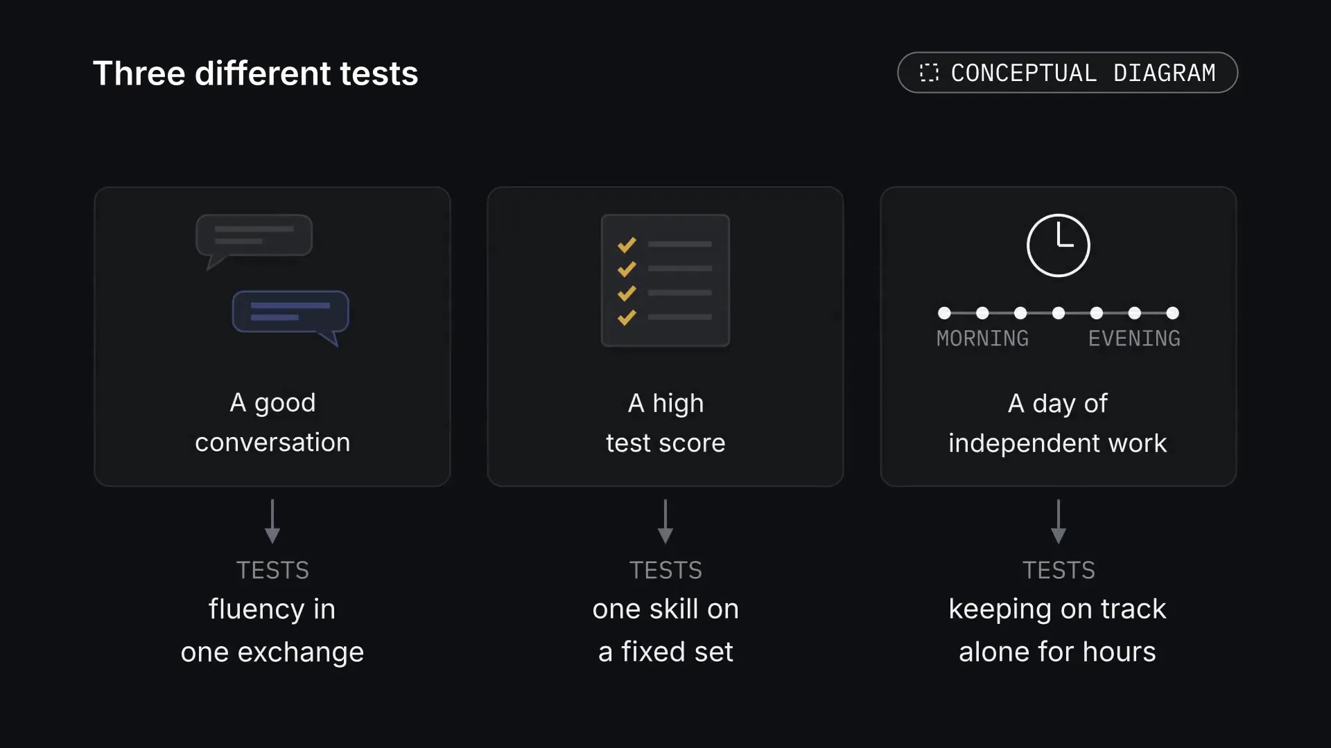
AGI, Artificial General Intelligence, usually means a system with broad intellectual abilities comparable to a person's. But a good conversation, a high test score and a day of independent work test different things.
FigureThree different tests. Three common impressions of an AI system test different abilities. Each says little about the other two. Conceptual diagram. Tap the picture to see it whole. The picture: Three cards side by side. A good conversation (two speech bubbles) tests fluency in one exchange; a high test score (a sheet of ticked answers) tests one skill on a fixed set; a day of independent work (a clock over a row of steps from morning to evening) tests keeping on track alone for hours.
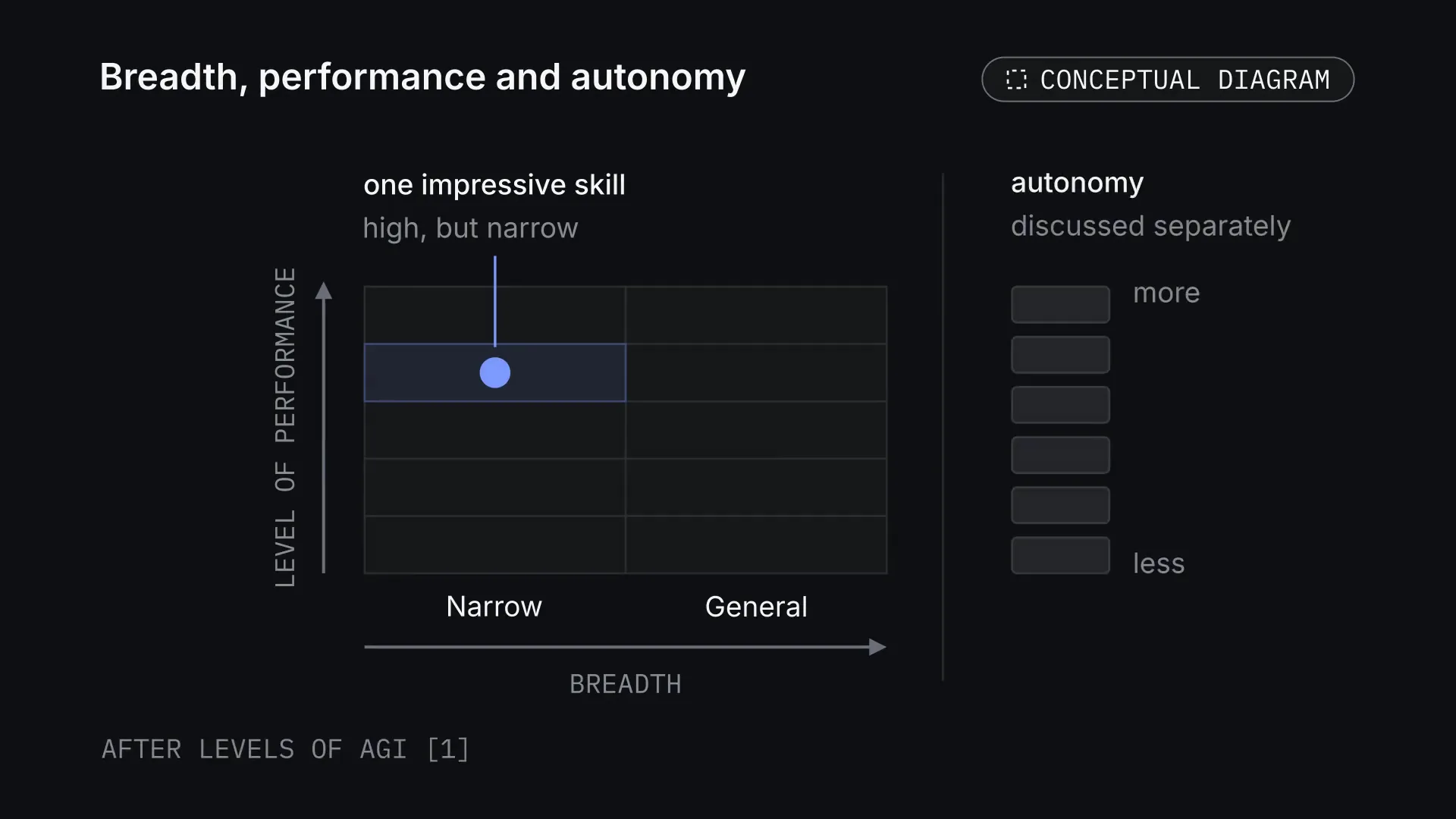
The paper Levels of AGI proposes looking at the breadth of abilities and the level of performance, and discussing autonomy separately. It is a useful starting point: one impressive skill is not enough to describe a whole system.[1]
FigureBreadth, performance and autonomy. After Levels of AGI [1]: breadth and level of performance form a grid, autonomy is discussed separately. One impressive skill sits high but in one narrow column. Conceptual diagram. Tap the picture to see it whole. The picture: A grid with two columns, narrow and general, along a breadth axis, and five rows up a level-of-performance axis. A single blue dot labelled 'one impressive skill, high but narrow' sits in an upper row of the narrow column. To the right, behind a divider, a separate vertical scale of six bars from less to more labelled 'autonomy, discussed separately'. Note: after Levels of AGI [1]. No real systems are placed.
For this diary it helps to keep four questions in view: how varied the tasks are, how reliable the result is, whether experience carries over to new conditions, and how much human involvement is needed. We write them down as a map of observations:
c=(B,R,T,A).
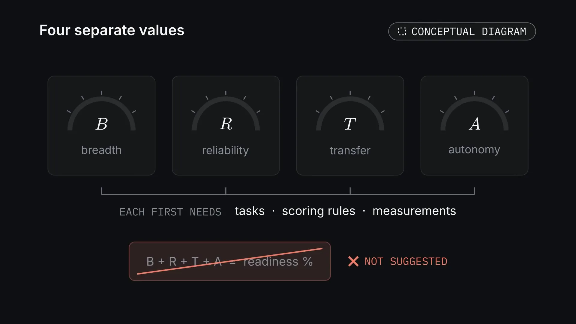
Here B is the breadth of tasks, R reliability, T transfer of experience and A autonomy. This is our explanatory scheme, not an accepted AGI index. We do not suggest adding these values up into a "percentage of intelligence readiness": each of them first needs tasks, scoring rules and measurements.
FigureFour separate values. B, R, T and A are four separate values, not parts of one score. Each first needs tasks, scoring rules and measurements. Conceptual diagram. Tap the picture to see it whole. The picture: Four cards with empty gauges for B (breadth), R (reliability), T (transfer) and A (autonomy), none with a needle. A bracket under all four reads 'each first needs tasks · scoring rules · measurements'. Below, a red box with 'B + R + T + A = readiness %' struck through, marked 'not suggested'.Walk-throughFour dimensions of ability · 18 sFigureFour dimensions of ability. Breadth of tasks, reliability, transfer of experience and autonomy are four separate questions. This scheme gives the system no scores and measures no percentage of AGI readiness. Conceptual diagram · 18 s. The picture: The formula c = (B, R, T, A) at the top. Below, four cards, each joined to its letter by a thin line, appear one by one as their letter in the formula turns blue: B Breadth — range of task types it handles; R Reliability — how consistently it succeeds; T Transfer — lessons carried to new tasks; A Autonomy — acting with no human step. No numbers.
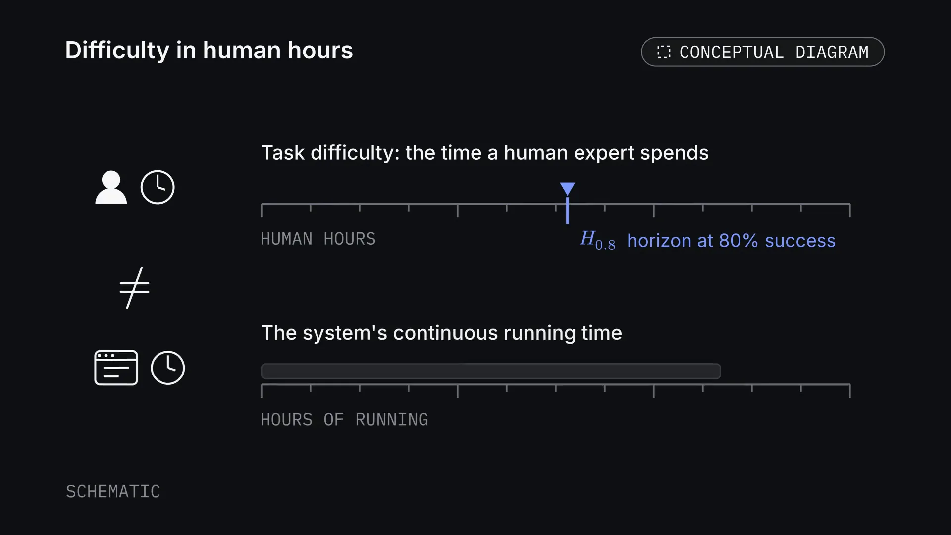
Another useful view is the task-difficulty horizon. METR estimates it by the time a human expert spends on a task. For example, the horizon at 80% success is the difficulty at which the system reaches that reliability according to the evaluation model. It is not the length of the system's continuous work.[2]
FigureDifficulty in human hours. The task-difficulty horizon is measured on the time a human expert spends on a task. It is not the length of the system's continuous work. Conceptual diagram. Tap the picture to see it whole. The picture: Two rulers, schematic and without numbers. Top, with a person and a clock: task difficulty as the time a human expert spends, in human hours, with a blue marker 'H_0.8, horizon at 80% success'. Bottom, with a computer window and a clock: the system's continuous running time, in hours of running, shown as a grey bar. A large ≠ stands between the two rows.
Hρ=sup{h:Pr(success∣h)≥ρ}.
In this explanatory notation h is the human duration of a task and ρ the chosen level of reliability. It assumes the probability of success falls as difficulty grows within the evaluated set. Different reliability requirements give different horizons.
Walk-throughThe task-difficulty horizon · 24 sFigureThe task-difficulty horizon. A teaching curve: at a 50% success requirement the horizon is 4 hours of human work, at 80% about 2.336 hours. This is not how long an AI works without stopping. Worked example · 24 s. The picture: The formula for H_ρ at the top. Below, axes: x is the hours a human expert needs for the task, 0 to 10; y is the probability of success, 0 to 1. A falling S-shaped blue curve on a panel. A violet dashed line at ρ = 0.5 meets it above h = 4, marked with a diamond; a second at ρ = 0.8 meets it above h ≈ 2.336. Two read-out cards on the right give both horizons; below them a legend gives the worked curve P(h) = 1/(1 + e^((h − 4)/1.2)).
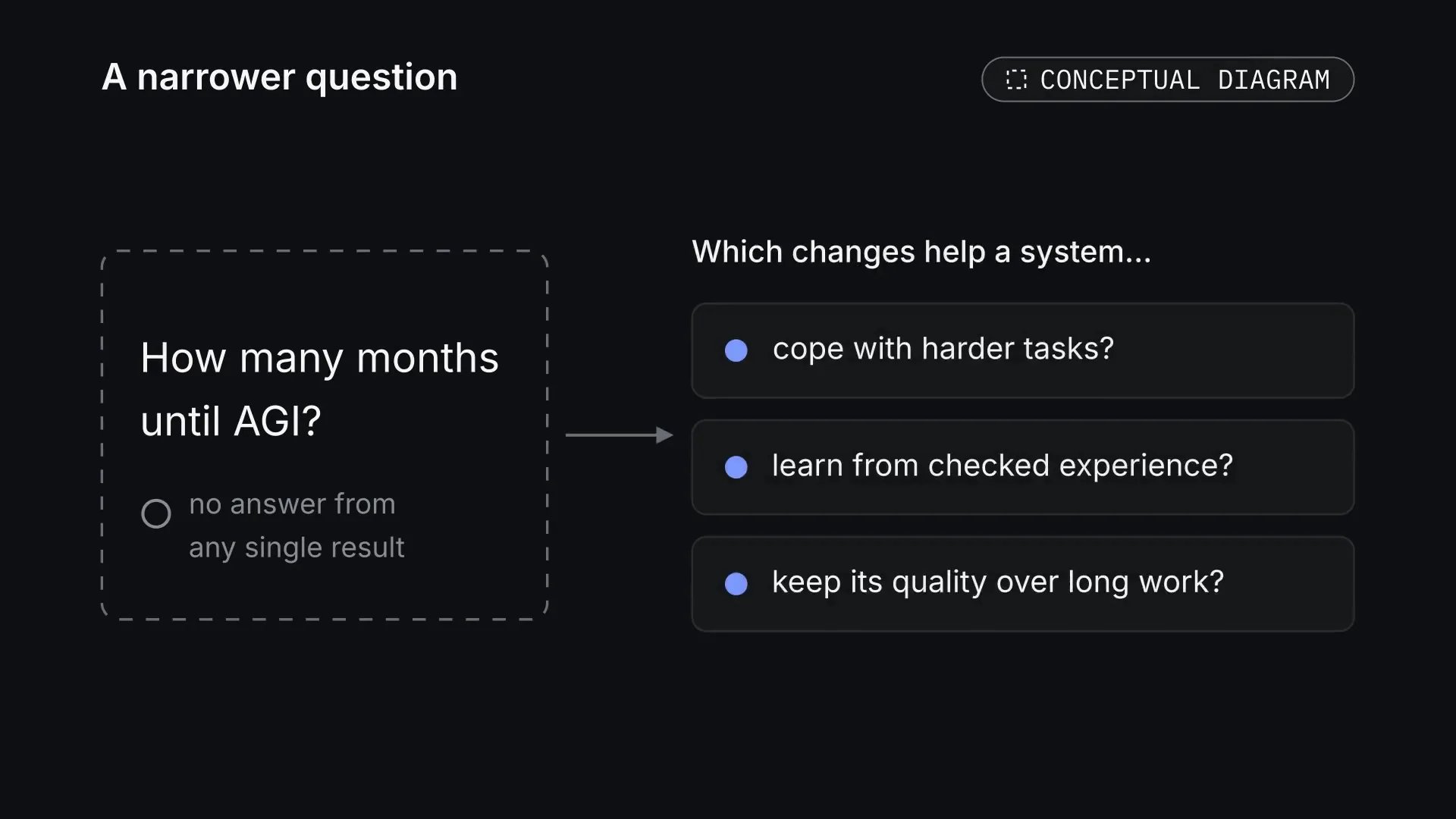
So the question "how many months are left until AGI?" does not yet have an answer that can be derived from any single result. Our research question is narrower and more concrete: which changes help a system cope with harder tasks, learn from checked experience and keep its quality over long work?
FigureA narrower question. No single result answers "how many months until AGI?". The research question is narrower: which changes help a system with harder tasks, checked experience and long work. Conceptual diagram. Tap the picture to see it whole. The picture: Left, a dashed card with the question 'How many months until AGI?' and the note 'no answer from any single result'. An arrow leads to the heading 'Which changes help a system…' and three cards: cope with harder tasks? learn from checked experience? keep its quality over long work?
What happens inside a language model
For an autoregressive LLM, generating an answer can be written as a sequence of conditional probabilities:
pθ(y1:n∣x)=i=1∏npθ(yi∣x,y<i).
x is the input context, yᵢ the next token and θ the model's parameters. A token can be a word, part of a word or another unit of text encoding. Each next piece depends on the available context and on the continuation already built.
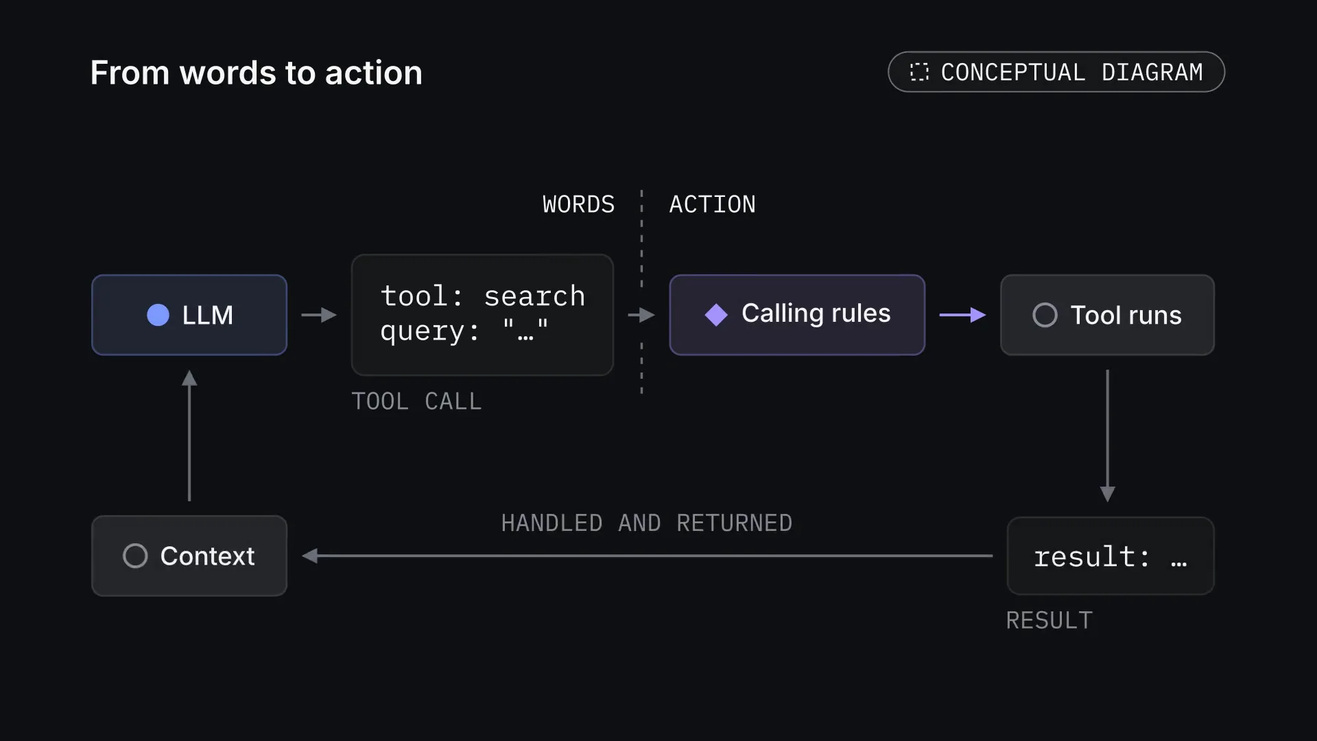
This formula describes the generation of a sequence. For the system to take an action in the outside world it also needs tools, rules for calling them and handling of their results.
FigureFrom words to action. Generating text is not yet acting. To act, a system needs tools, rules for calling them and handling of their results. Conceptual diagram. Tap the picture to see it whole. The picture: A loop. The LLM (blue) writes a tool call card ('tool: search, query: …'). A dashed boundary separates words from action. The call passes calling rules (violet) to 'Tool runs'; the result card ('result: …') is handled and returned to the context, which feeds the LLM again.Walk-throughGenerating a sequence of tokens · 22 sFigureGenerating a sequence of tokens. A worked example: the tokens ready, for and review extend the context one after another. Conditional probabilities of 0.6, 0.5 and 0.8 give 0.24 for the whole chosen sequence. The bottom line shows the product being built up step by step. Worked example · 22 s. The picture: The product formula at the top. Below, the prompt tokens 'The report is' in boxes. Three answer tokens appear one at a time — 'ready', 'for', 'review' — each in a blue-tinted box with its probability under it (0.6, 0.5, 0.8), while a thin green bracket labelled 'context' grows to cover the prompt and every earlier token, with an arrow into the next token. A card at the bottom builds 0.6 × 0.5 × 0.8 = 0.24.
One of the main mechanisms of the Transformer is attention. In the simplified notation for a single head it looks like this:
Attention(Q,K,V)=softmax(dkQKT)V.
The matrices Q, K and V hold queries, keys and values. Matching queries against keys sets the weights by which the values are mixed. Scaling by the square root of the dimension dₖ helps keep the size of the scores in check before the softmax. This is a computational mechanism, not a measure of human attention.[3]
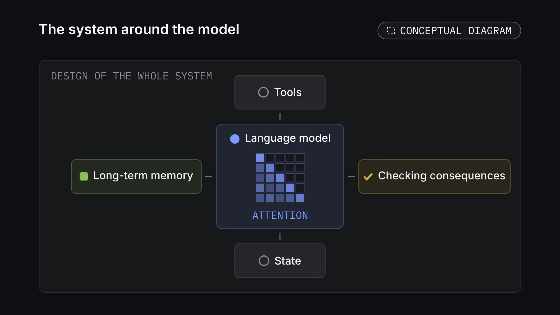
Attention on its own does not organise a project's long-term memory or the checking of an action's consequences. Those functions belong to the design of the whole system around the model.
FigureThe system around the model. Attention works inside the model. Long-term memory, checking consequences, tools and state belong to the design of the whole system around it. Conceptual diagram. Tap the picture to see it whole. The picture: A large panel labelled 'design of the whole system'. In the centre a blue card 'Language model' with a small causal attention grid inside, labelled 'attention'. Around it, joined by short lines: Long-term memory (green) on the left, Checking consequences (ochre) on the right, Tools above, State below.Walk-throughAttention, step by step · 28 sFigureAttention, step by step. One attention head on three made-up tokens: the score matrix, scaling, a row-by-row softmax and mixing the values V. Numbers on screen are rounded to two places; the computation uses more precision. Worked example · 28 s. The picture: The attention formula at the top. Below, each matrix sits on a card named above it, and thin arrows labelled multiply, ÷ √2 and softmax lead from one card to the next. Q times K transpose gives the 3 × 3 score matrix [[1,0,1],[0,1,1],[1,1,2]]. Divided by √2 it becomes [[0.71,0,0.71],[0,0.71,0.71],[0.71,0.71,1.41]]. Softmax row by row, each row framed in turn, gives [[0.40,0.20,0.40],[0.20,0.40,0.40],[0.25,0.25,0.50]], each row summing to 1. Times V it gives the 3 × 2 result [[0.80,0.60],[0.60,0.80],[0.75,0.75]].
The idea behind Sapphire
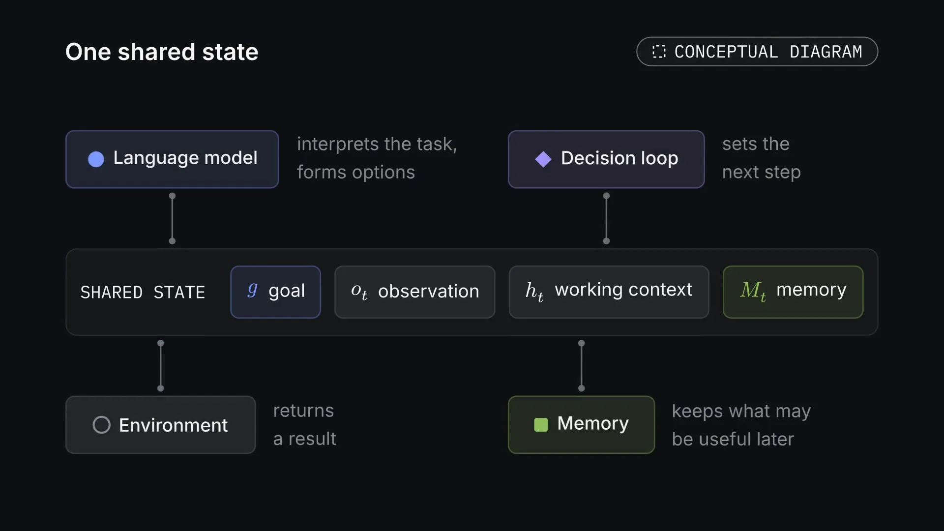
We are studying a single architecture in which generation, decision-making and work with experience are linked by a shared state. The language model helps interpret the task and form options. The decision loop sets the next step. The environment returns a result. Memory keeps what may be useful later.
FigureOne shared state. One shared state links the parts. The language model interprets the task and forms options, the decision loop sets the next step, the environment returns a result, and memory keeps what may be useful later. Conceptual diagram. Tap the picture to see it whole. The picture: A wide band 'shared state' holding four chips: g goal (blue), o_t observation, h_t working context, M_t memory (green). Joined to it by short connectors: above, Language model (interprets the task, forms options) and Decision loop (sets the next step); below, Environment (returns a result) and Memory (keeps what may be useful later).
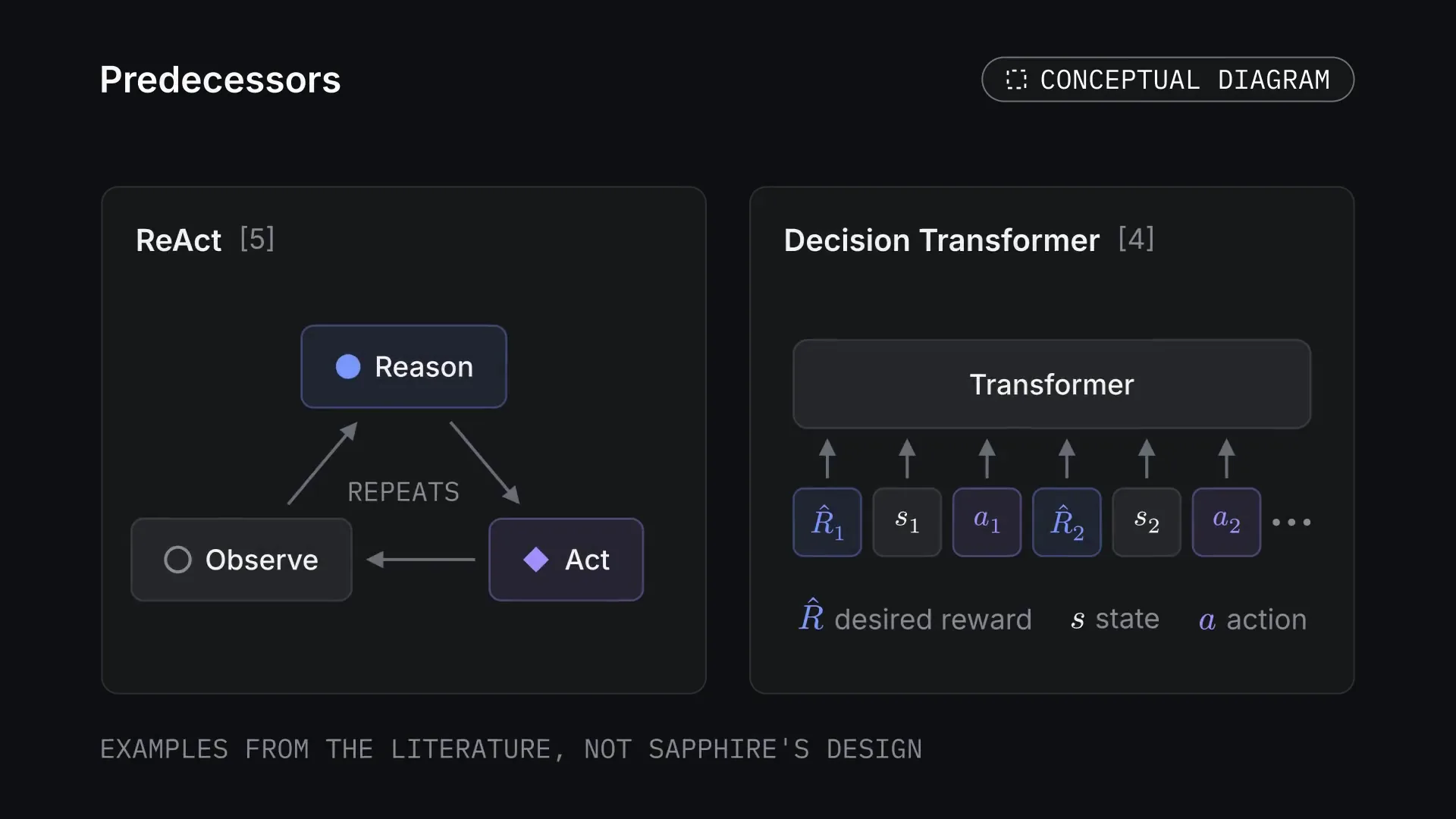
By Decision models in this entry we mean the functional loop that chooses actions. The specific algorithm cannot be read from that name. Language models and decision models also do not have to be mutually exclusive architectures: Decision Transformer, for example, applies a Transformer to sequences of states, actions and desired reward. This is an example from the literature, not a statement that Sapphire uses it.[4]
To describe our idea, we introduce the state of the system:
stst+1=(g,ot,ht,Mt),=Fθ,ϕ(st,at,ot+1).
g is the goal, oₜ the current observation, hₜ the system's working context, Mₜ long-term memory and aₜ the action. In the accompanying diagram θ stands for the language model's weights and φ for the settings of the control loop, the harness. This notation describes the system loosely; it does not claim a separate trained decision model exists. The working context here should not be confused with the hidden state of a single neural-network layer.
The function F describes the whole system's transition to the next step. In the diagram it passes through interpretation, choosing an action, executing it and checking the result. This is a conceptual formalisation, not a published implementation specification.
Loops of this kind have predecessors. In ReAct a language model alternates reasoning and actions, using the results of its interaction with the environment. So the research value of Sapphire has to be judged by what our particular organisation of the loop gives in practice.[5]
FigurePredecessors. Two examples from the literature: ReAct alternates reasoning and actions; Decision Transformer applies a Transformer to sequences of desired reward, state and action. They are examples, not Sapphire's design. Conceptual diagram. Tap the picture to see it whole. The picture: Two panels. ReAct [5]: a repeating cycle Reason → Act → Observe. Decision Transformer [4]: a row of tokens R̂1, s1, a1, R̂2, s2, a2 … each feeding up into a Transformer block, with a legend R̂ desired reward, s state, a action. Note below: examples from the literature, not Sapphire's design.FigureThe architecture of Sapphire. Conceptual architecture: the state holds the goal, the observation, the working context and memory. After an action the environment returns a result; the check shapes the next step and what is written to memory. There is an exit when the goal is reached or the budget is spent. Conceptual diagram · 32 s. The picture: Two formulas at the top: s_t = (g, o_t, h_t, M_t), labelled goal, observation, context, memory, and s_{t+1} = F_{θ,φ}(s_t, a_t, o_{t+1}). Below, tinted cards for LLM (blue), Choose action (violet), Tool & environment (grey), Verify (ochre) and Update context (grey) joined in a loop by thin arrows. A green Memory card in the middle sends a 'read' arrow to Choose action and receives an 'update' arrow from Verify. An Exit card on the right is reached from Verify: goal reached or budget spent.
To explain the choice of the next step, we can use this objective:
The system considers the allowed actions, estimates their expected usefulness U and takes cost into account. The coefficient λ sets the weight of costs. The formula states a design principle: usefulness has to be weighed against expense. It does not mean a separately trained usefulness function is already implemented or predicts outcomes accurately.
Walk-throughChoosing the next action · 24 sFigureChoosing the next action. Teaching scores with λ = 0.8: ask the user, 4.6; query the API, 7.4; search memory, 5.6. Deleting, which is not allowed, is excluded in advance. These scores are not measurements of Sapphire. Worked example · 24 s. The picture: The formula at the top. A table on a panel lists four actions with usefulness U and cost. 'Delete old records' is framed in clay red, dimmed and tagged with a cross as not allowed before any score is computed. For the other three, a violet bar shows U − 0.8 × Cost: Ask the user 4.6, Query the API 7.4, Search memory 5.6. The 7.4 row is framed in violet and its bar turns solid: chosen.
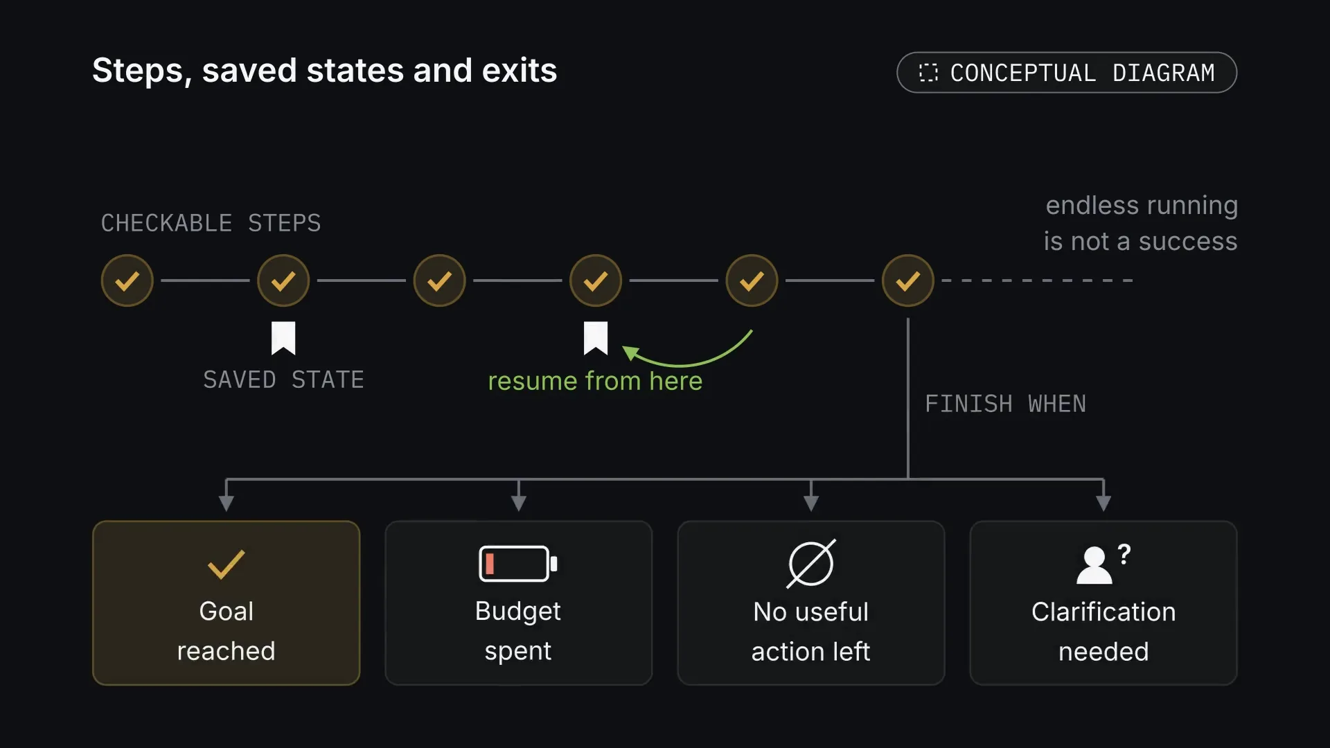
By continuous work we mean the ability to move from one checkable step to the next and to resume work from a saved state. Such a process has to be able to finish when the goal is reached, the budget is spent, no useful action is left or clarification is needed. Endless execution is not a success in itself.
FigureSteps, saved states and exits. Continuous work moves between checkable steps and can resume from a saved state. It must be able to finish: goal reached, budget spent, no useful action left, or clarification needed. Conceptual diagram. Tap the picture to see it whole. The picture: A row of six ticked step circles, labelled 'checkable steps', trailing off in a dashed line marked 'endless running is not a success'. Bookmarks under two steps mark saved states; a green arrow points back to one: 'resume from here'. From the last step a branch labelled 'finish when' leads to four cards: Goal reached (tick), Budget spent (empty battery), No useful action left (empty set), Clarification needed (person with a question mark).
Why a system needs long-term memory
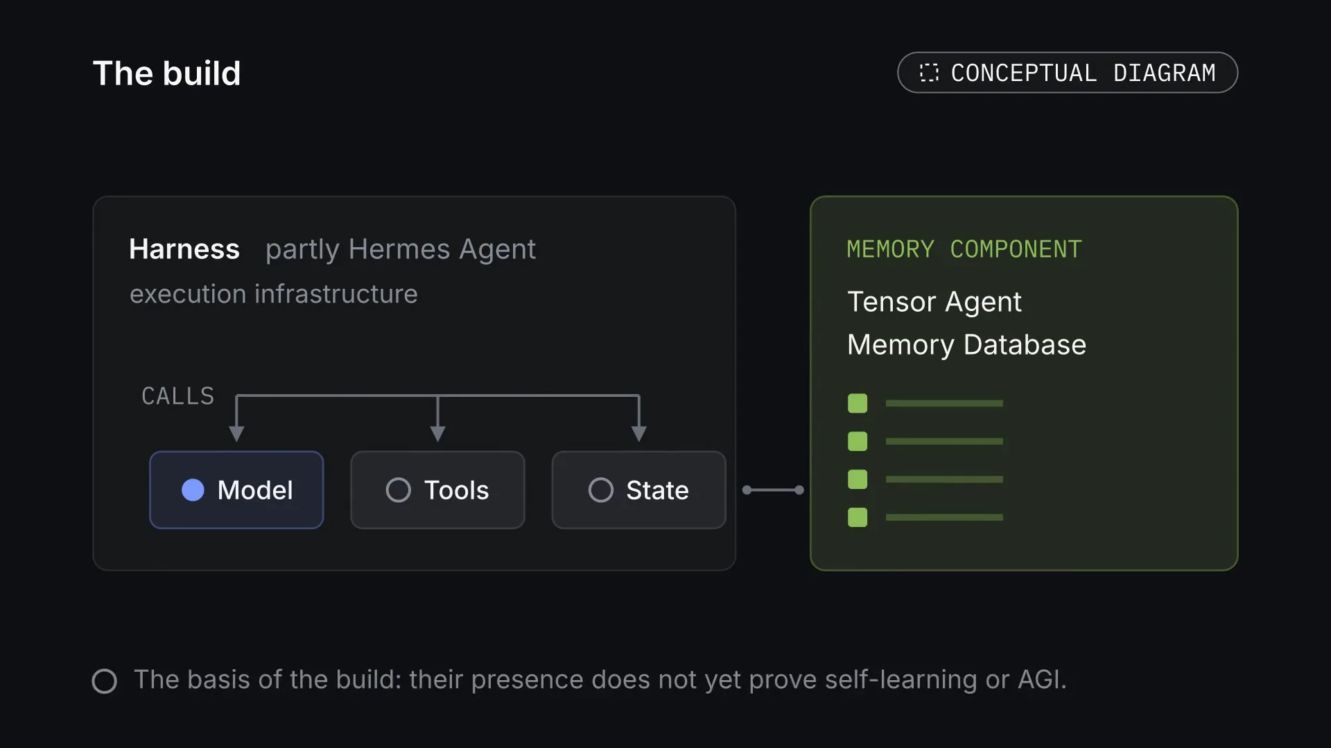
In our current work we use a component the team calls Tensor Agent Memory Database, and part of the Hermes Agent agent harness. A harness here means the execution infrastructure: how calls to the model, the tools and the state are organised. These components are the basis of the build; their presence does not yet prove self-learning or AGI.
FigureThe build. The build uses part of the Hermes Agent harness and a memory component the team calls Tensor Agent Memory Database. They are the basis of the build, not proof of self-learning or AGI. Conceptual diagram. Tap the picture to see it whole. The picture: Left, a frame 'Harness, partly Hermes Agent, execution infrastructure' in which a 'calls' line branches to Model (blue), Tools and State. Right, joined to State, a green card 'memory component: Tensor Agent Memory Database' with a few record rows. A quiet note below: the basis of the build; their presence does not yet prove self-learning or AGI.
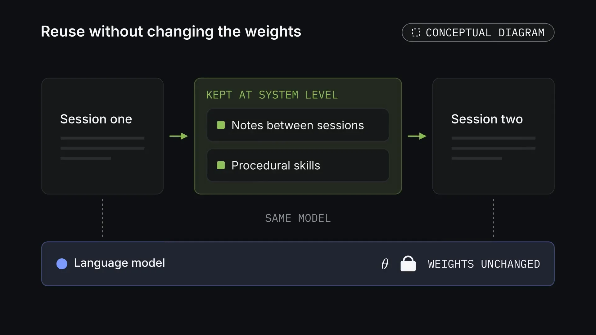
The official Hermes documentation describes notes kept between sessions and procedural skills. That is important context for us: experience can be reused at the level of the system, without changing the language model's weights.[6]
FigureReuse without changing the weights. Experience can be reused at the level of the system: notes between sessions and procedural skills carry from one session to the next, while the model's weights stay unchanged. Conceptual diagram. Tap the picture to see it whole. The picture: Session one → a green panel 'kept at system level' with Notes between sessions and Procedural skills → Session two. Below, both sessions connect by dashed lines ('same model') to one blue band: Language model, θ with a padlock, 'weights unchanged'.
One way to look for a fitting memory is to compare the query's vector with the vectors of the records:
qₜ represents the current query and eₘ a memory record. For cosine similarity both vectors must be non-zero. TopK returns the few records with the highest similarity. This illustrates a possible search; it is not a statement about the internal algorithm of the named database.
A similar record, however, may be wrong, out of date or valid for one project only. So useful memory needs a source, a time, a scope and a way to be corrected. Similarity helps find a record; whether it is true is checked separately.
Walk-throughSearching long-term memory · 24 sFigureSearching long-term memory. A teaching search by cosine similarity gives about 0.99, 0.71 and −0.39. Of the two records found, one has to be rejected because of an unconfirmed source, its age and a different API version. All records and dates are made up. Worked example · 24 s. The picture: Two formulas at the top left; below them, on an inset, a small plane with a blue query arrow q and green arrows e1, e2, e3. On the right, three cards with similarity 0.99 'Orders sync by API polling', 0.71 'Webhooks retry every 5 min' and −0.39 'Meeting notes template'. The top two turn green as recalled; the third fades. Then each recalled card shows its source, date and scope: the first a verified run log from 2026-09-14 for Client A, API v2 (ochre tick); the second an unchecked chat message from 2024-03-02 for API v1 only (red cross).
To explain how checked experience is written down, a rule helps:
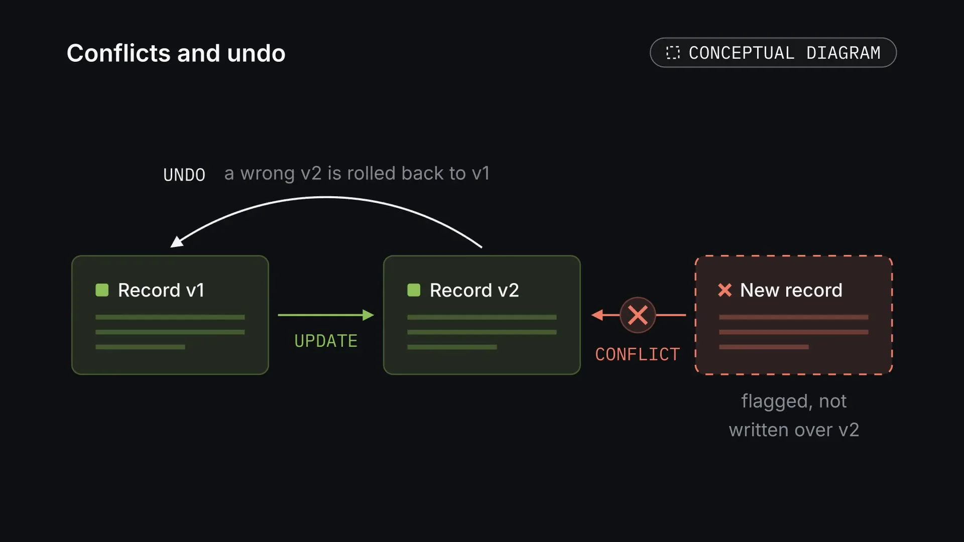
Upsert means adding or updating a record, Verified the result of a given check. A real system will also need conflict handling and a way to undo wrong records. The formula states the intended principle, not a guarantee of error-free memory.
FigureConflicts and undo. Writing memory needs more than an update rule: a conflicting record has to be caught, and a wrong record has to be undone. Conceptual diagram. Tap the picture to see it whole. The picture: Record v1 → (update) → Record v2, both green cards. A dashed red 'New record' pushes toward v2 but is stopped by a red cross labelled 'conflict': flagged, not written over v2. A curved arrow from v2 back to v1 is labelled 'undo: a wrong v2 is rolled back to v1'.Walk-throughWriting down checked experience · 22 sFigureWriting down checked experience. The check first rejects an unconfirmed record, then accepts a change to the existing record about sync. The number of records stays at three: Upsert updates the right key instead of creating a duplicate. Worked example · 22 s. The picture: The cases formula at the top left. Below it a flow of flat cards joined by thin arrows: a dashed slot for a new record on the left, an ochre Verify box in the middle and, on the right, memory with three records: Client A · sync — webhook (v1), Invoices — PDF, monthly (v1), Reports — every Monday (v1). A candidate 'Client A · export: FTP upload' gets a red cross ('not verified') and drops below the check as a faded 'dropped' card; memory is unchanged. A second candidate 'Client A · sync: API polling, 15 min' gets an ochre tick and goes on into the matching record, which now reads 'API polling, 15 min' with version v2: updated, not duplicated.
In what sense a system can learn
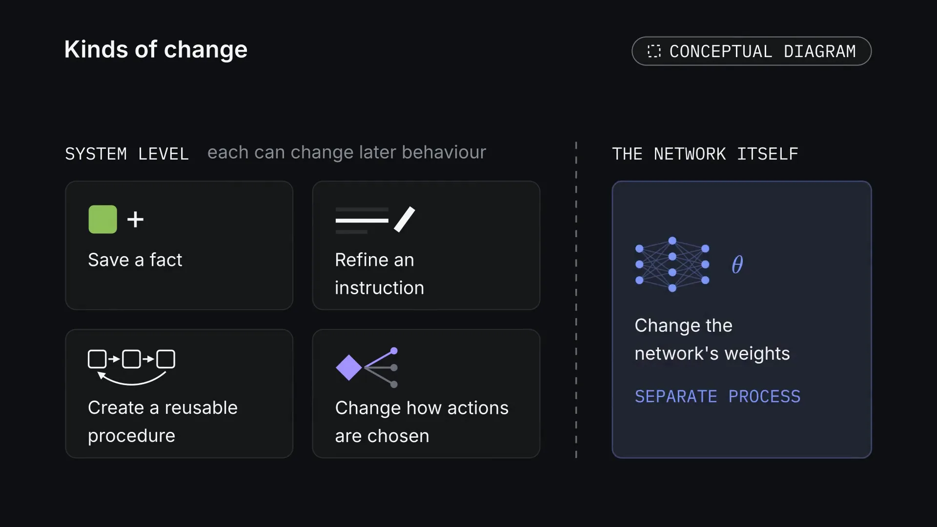
"Self-learning" has several meanings here. A system can save a fact, refine an instruction, create a reusable procedure or change how it chooses actions. Each of these can change its later behaviour. Changing the parameters of the neural network itself is a separate process.
FigureKinds of change. At system level, a system can save a fact, refine an instruction, create a reusable procedure or change how it chooses actions. Changing the network's weights is a separate process. Conceptual diagram. Tap the picture to see it whole. The picture: Under 'system level, each can change later behaviour', four cards with pictograms: Save a fact (green square and plus), Refine an instruction (lines and a pen), Create a reusable procedure (three linked boxes with a loop back), Change how actions are chosen (a violet diamond with branching options). Behind a dashed divider, under 'the network itself', a blue card with a small neural network and θ: Change the network's weights, a separate process.
The first line shows memory changing while the LLM's weights stay the same. The second shows the usual gradient update: η sets the step size, L is the loss function and D_checked the checked training data. The second line is there to explain the difference; with it we do not claim that Sapphire already retrains its weights on its own.
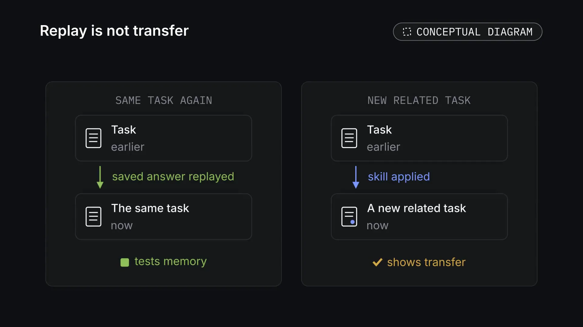
What matters to us is the observable result: after useful experience the system should do better on relevant new tasks. Replaying a saved answer tests memory but does not yet show that a skill carried over.
FigureReplay is not transfer. Replaying a saved answer on the same task tests memory. Only a skill applied to a new, related task shows that something carried over. Conceptual diagram. Tap the picture to see it whole. The picture: Two panels. Left, 'same task again': a task card marked earlier, a green arrow 'saved answer replayed' down to 'the same task', now; verdict with a green square: tests memory. Right, 'new related task': a task card marked earlier, a blue arrow 'skill applied' down to 'a new related task', now, whose page icon differs by one blue dot; verdict with an ochre tick: shows transfer.FigureSystem memory and weight training. On the left, memory M changes while the weights θ stay the same; on the right, gradient training is explained. The teaching curve uses L(θ) = (θ − 2)² + 0.5 and η = 0.3. This video does not claim Sapphire trains its own weights. Conceptual diagram · 30 s. The picture: Two columns. Left, 'Memory update': M_{t+1} ≠ M_t, θ_{t+1} = θ_t; a stack of memory cards gains a new green-edged card while a grid of violet weight cells stays the same, labelled 'weights unchanged'. Right, 'Weight training': θ_{k+1} = θ_k − η ∇L(θ_k; D_checked); a dot steps three times down a U-shaped error curve, leaving faded dots behind, η = 0.3. A note says this is explained, not claimed as working in Sapphire.
What zeros and ones can explain
Binary notation makes it easy to show how a system narrows its set of actions. Take four example actions in a fixed order: read, delete, verify, write. The availability mask might look like this:
bt=(1,0,1,1),(1011)2=1110.
A one means the action is available at the current step, a zero that it is excluded. The value 11 is the ordinary decimal form of this bit sequence. What the mask means is set by which position stands for which action.
Walk-throughA binary mask of actions · 18 sFigureA binary mask of actions. The order of actions is fixed: read, delete, verify, write. The mask 1011 excludes deleting. As a binary number it equals 11 in decimal. Worked example · 18 s. The picture: The formula b = (1, 0, 1, 1) at the top left. Below it a small table with the rows action, bit and place: four flat chips read, delete, verify, write, with the bits 1, 0, 1, 1 under them. Read, verify and write turn blue (allowed); the delete chip turns red with a cross and dims: blocked. Place values ×8, ×4, ×2, ×1 appear under the bits and the line (1011)₂ = 1·8 + 0·4 + 1·2 + 1·1 = 11₁₀ builds at the bottom.
If, before the mask is applied, the probabilities of actions are given by the distribution π, the available options can be renormalised:
π(ai∣st)=∑jbjπ(aj∣st)biπ(ai∣st).
With a positive denominator the excluded action gets zero probability, and the rest again add up to one. If the denominator is zero the formula does not apply: the system has to take a planned exit, such as stopping or asking for clarification.
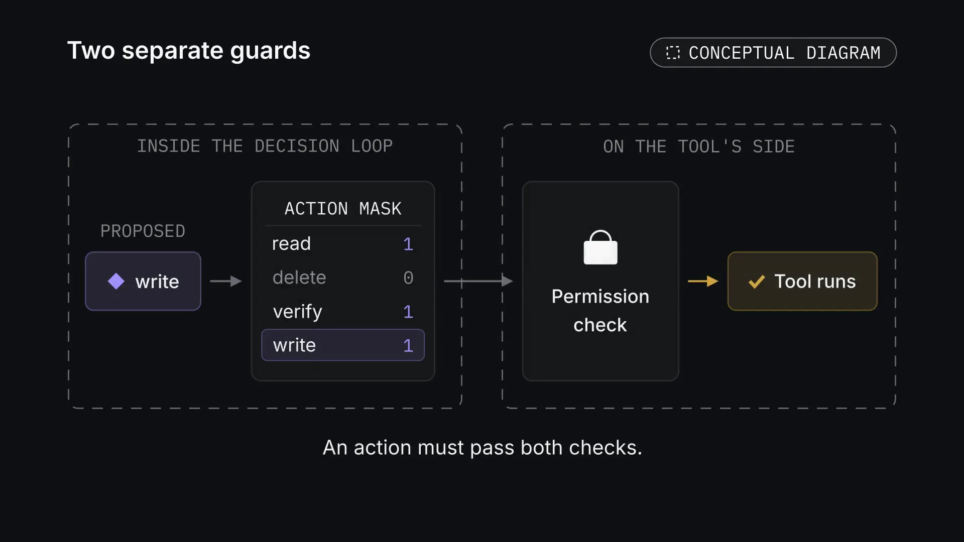
This is a teaching example of controlling actions. Such a mask is not proof of learning on its own, and it does not replace the permission check on the side of the tool being run.
FigureTwo separate guards. The action mask works inside the decision loop; the permission check works on the side of the tool. A proposed action has to pass both. Conceptual diagram. Tap the picture to see it whole. The picture: Two dashed regions side by side. 'Inside the decision loop': a violet chip 'write' labelled proposed, an arrow to an action mask card listing read 1, delete 0 (greyed), verify 1, write 1, with the write row highlighted. An arrow crosses into 'on the tool's side': a card with a padlock, 'Permission check', then an ochre arrow to 'Tool runs' with a tick. Below: an action must pass both checks.Walk-throughMasking probabilities · 24 sFigureMasking probabilities. The mask turns the distribution (0.1, 0.6, 0.2, 0.1) into (0.25, 0, 0.5, 0.25). The edge case of a zero denominator is shown separately: division does not apply, and the process needs a planned exit. Worked example · 24 s. The picture: The masking formula at the top left. Below it, on an inset, flat bars for read, delete, verify, write at 0.1, 0.6, 0.2, 0.1. The mask ×1, ×0, ×1, ×1 appears under them; the delete bar drops to 0. On the right the sum of what is left, 0.4, is worked out, and the bars rescale to 0.25, 0, 0.5, 0.25 in violet. Finally a red case: if every allowed probability is 0 the sum is 0, division is undefined, and thin arrows lead to two exits: stop, or ask the user for clarification.
A concrete scenario to test the idea
In the accompanying illustration the requirements document changes: webhook sync is replaced by an API request every 15 minutes. The list has three tasks that involve the webhook and one more task unrelated to the integration.
The system first rewrites the three related tasks for the new way of syncing. Then the check finds an exception: under Client B's terms, its webhook has to keep working. The wrong change to that task is undone, and the saved rule is refined to include the exception. The other two tasks stay switched to the API request.
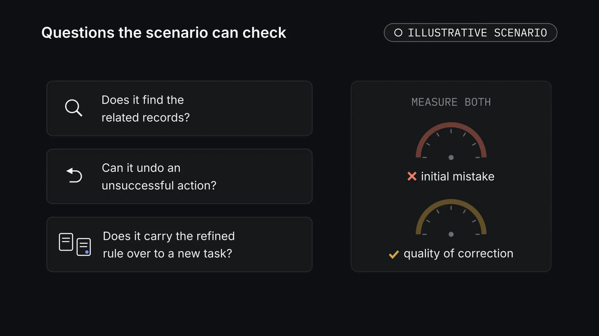
An example like this lets us ask checkable questions: does the system find the related records, can it undo an unsuccessful action, and does it carry the refined rule over to a new task? It matters to measure both the initial mistake and the quality of its correction.
FigureQuestions the scenario can check. The illustrative scenario lets us ask checkable questions. Both the first mistake and how well it is corrected need measuring. Illustrative scenario. Tap the picture to see it whole. The picture: Three question cards with small pictograms: a magnifier, 'Does it find the related records?'; an undo sign, 'Can it undo an unsuccessful action?'; two pages, 'Does it carry the refined rule over to a new task?'. On the right a panel 'measure both' with two empty dials without readings: one clay with a cross, 'initial mistake'; one ochre with a tick, 'quality of correction'.
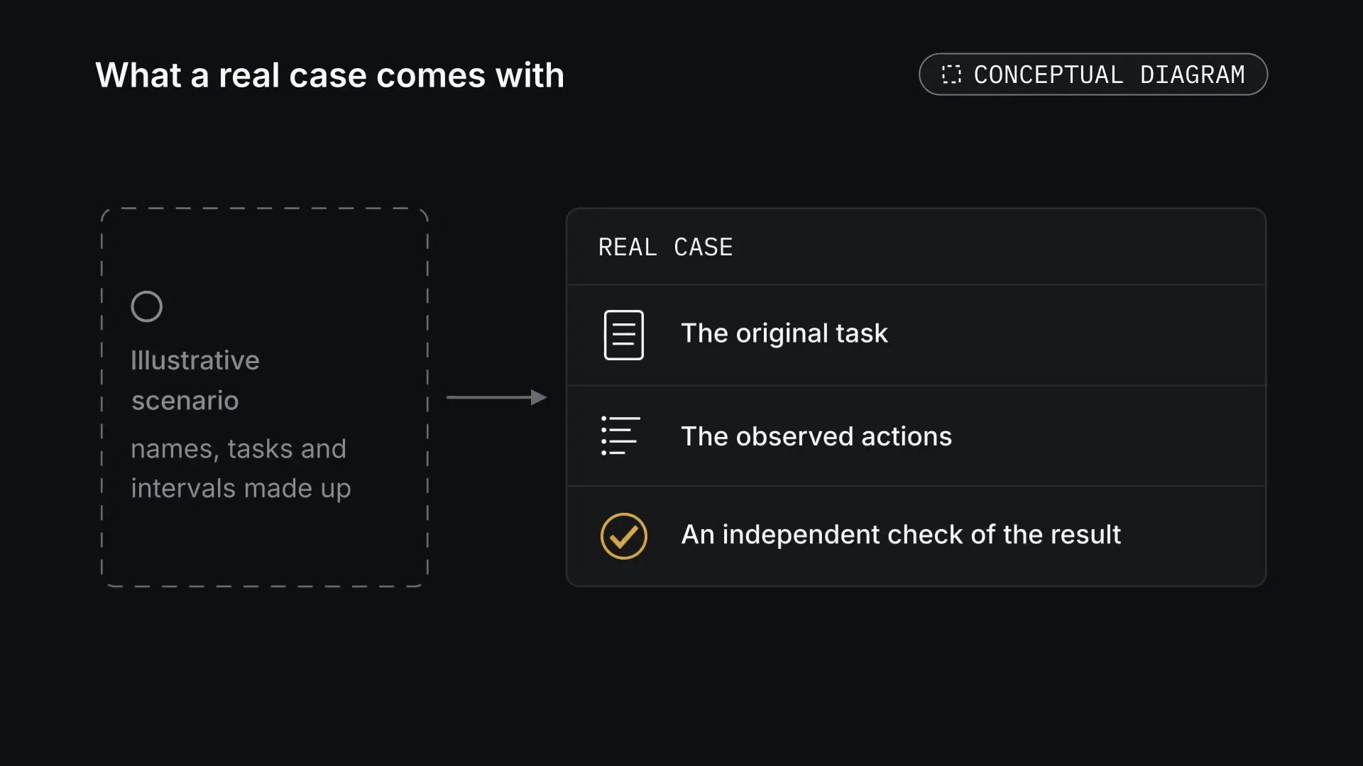
This is an illustrative scenario, not a description of an experiment that was run. The client names, tasks and intervals here are made up. A real case has to come with the original task, the observed actions and an independent check of the result.
FigureWhat a real case comes with. The scenario in this article is made up. A real case has to come with the original task, the observed actions and an independent check of the result. Conceptual diagram. Tap the picture to see it whole. The picture: On the left a dashed card with a ring: illustrative scenario, names, tasks and intervals made up. An arrow leads to a record headed 'Real case' with three joined rows: a page icon, the original task; a log icon, the observed actions; a ringed ochre tick, an independent check of the result.FigureA changed requirement and an exception. An illustrative scenario: after the requirement changes, the system first changes three tasks, then finds the exception for Client B, restores its webhook and refines the rule. This is an example of correcting a mistake, not a recording of a product feature. Illustrative scenario · 32 s. The picture: Top left, a requirement card: 'Sync by webhook' struck out, replaced by 'Poll the API every 15 min'. Below, a list of open tasks T-14 to T-17 as flat rows. The three that mention webhooks turn blue as outdated and are all rewritten for polling, T-16 for Client B too. On the right a check list ticks T-14 and T-15, and a green memory card saves the rule 'Sync: API polling every 15 min'. Then the check on T-16 fails (red cross: Client B's contract needs a webhook) and its row turns red; it is restored to 'Client B webhook alerts', marked 'restored' with an ochre tick, and the rule card gains 'except Client B: webhook stays'.
The third stage of the work
According to the team's report of 28 October 2026, Sapphire is at its third stage: assembling the components into one project. The animations in this article explain the idea; they are not a recording of Sapphire at work. This publication gives no numerical results of internal trials.
The plan of work can be shown in four stages:
Stage
What it involves
What lets us move on
Hypothesis
Define the tasks and the research hypothesis
There are observable criteria of success
Components
Prepare the generation, action and memory components
Their roles and ways of working together are clear
Single loop
Assemble the single loop
State and results pass between the components
Comparative trials
Run comparative trials
There are reproducible results and an analysis of errors
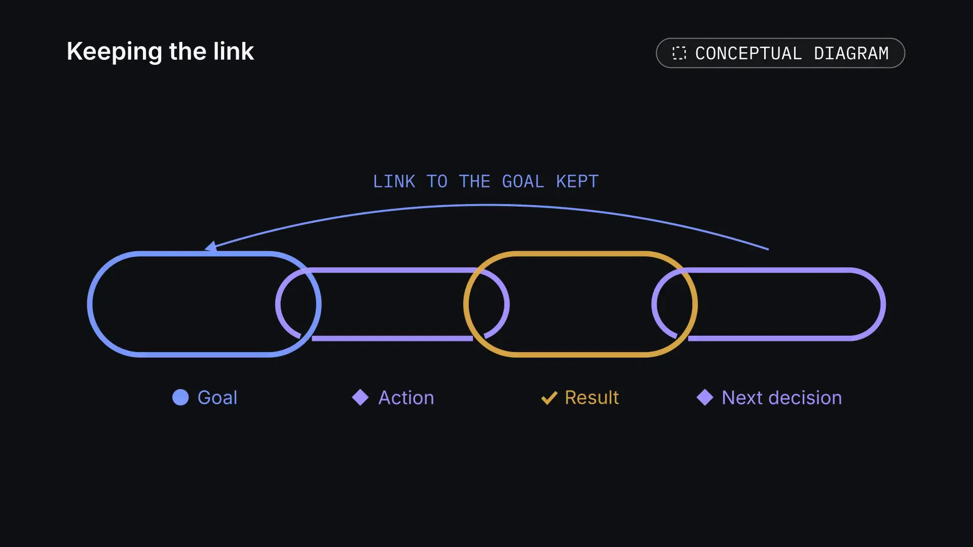
This is a map of the project's content; it does not replace a report that each step is complete. The main question of the current integration is whether the single loop can keep a useful link between the goal, the action, the result and the next decision.
FigureKeeping the link. The question of the current integration: can the single loop keep the goal, the action, the result and the next decision linked, without losing the goal? Conceptual diagram. Tap the picture to see it whole. The picture: Four interlocking chain links in a row, labelled below: Goal (blue disc), Action (violet diamond), Result (ochre tick), Next decision (violet diamond). A thin blue arrow arcs from the last link back to the first, labelled 'link to the goal kept'.FigureThe project's third stage. As the team reports, the current stage is assembling the single loop. The four nodes are a map of the work's content; they are not a scale of AGI readiness. Team status report · 18 s. The picture: Four flat cards in a row joined by thin arrows: Hypothesis, Components, Unified loop, Comparative trials, with names only and no numbers. The Unified loop card is tinted blue and labelled 'current stage', 'as reported by the team'; the Comparative trials card is labelled 'next'. A note reads 'order of stages only · no dates · no percentages'. There are no progress bars.
What published experiments already show
In the 2023 Reflexion study the authors compared plain generation with a system that uses feedback and text memory. Their Table 1 gives these results for Python:[7]
Benchmark
Base GPT-4
Reflexion
Difference
HumanEval
80.1%
91.0%
+10.9 pp
MBPP
80.1%
77.1%
−3.0 pp
These are historical results of specific configurations, not measurements of Sapphire. The metric is called pass@1, but the Reflexion process includes internal checking and corrections before the final score, and the compute costs differ. A gain on one set sits next to a loss on another.
FigureA published comparison: Reflexion. A comparison published in 2023, Python, pass@1: HumanEval 80.1% → 91.0%; MBPP 80.1% → 77.1%. These are results of the Reflexion paper, not of Sapphire; the checking processes and compute costs differ. Published experiment · 2023 · 26 s. The picture: A flat horizontal bar chart on a panel, 0 to 100 % scale with thin gridlines. HumanEval: GPT-4 80.1 % (grey bar, ring marker), Reflexion 91.0 % (green bar, square marker), difference +10.9 pp in ochre with a tick. MBPP: GPT-4 80.1 %, Reflexion 77.1 %, difference −3.0 pp in red with a cross. A note reads 'Not Sapphire results; different verification processes and costs', and the source line cites arxiv.org/html/2303.11366v4, Table 1.
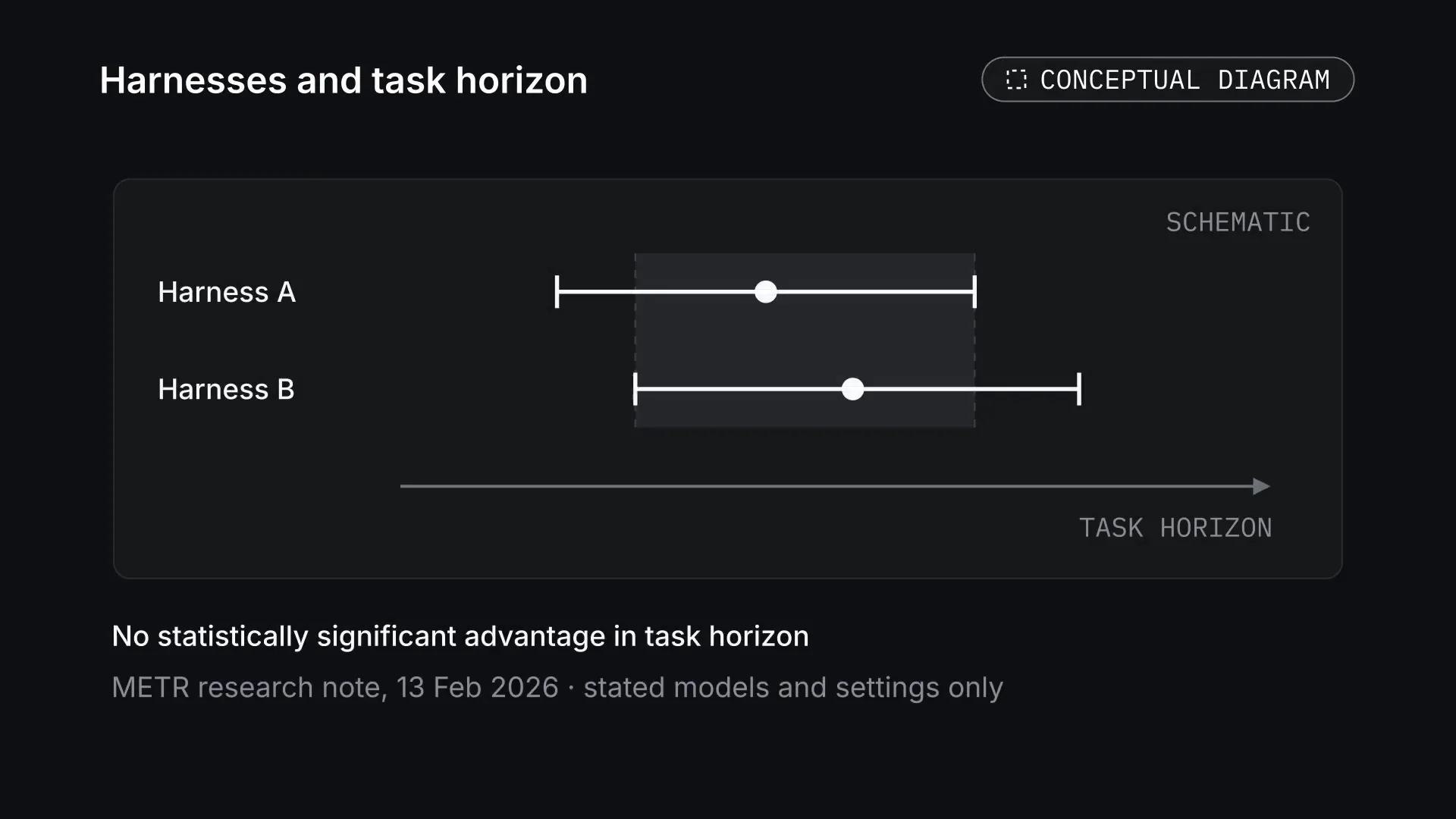
There is also a more recent test of what an agent harness contributes. In a METR research note of 13 February 2026, comparing Codex and Claude Code with the harnesses METR uses, on GPT-5 and Opus 4.5, showed no statistically significant advantage in task horizon. This is a limited experiment with the stated models and settings, not a general conclusion that harnesses are useless.[8]
FigureHarnesses and task horizon. Schematic, not METR's data: overlapping intervals show what no statistically significant advantage looks like. The METR note covers only the stated models and settings. Conceptual diagram. Tap the picture to see it whole. The picture: A panel marked 'schematic'. Two horizontal interval bars with a central dot, 'Harness A' and 'Harness B', overlap over a shaded band; below them an axis arrow 'task horizon' with no ticks or numbers. Under the panel: No statistically significant advantage in task horizon; METR research note, 13 Feb 2026, stated models and settings only.
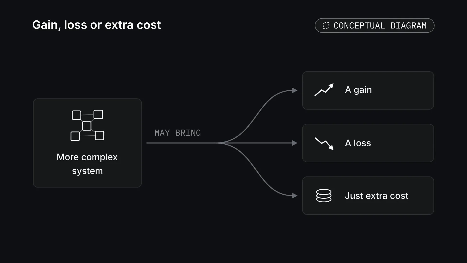
What we take from these papers is a research hypothesis: the quality of feedback, memory and loop control deserves to be measured on its own. A more complex system may bring a gain, a loss or just extra cost.
FigureGain, loss or extra cost. Adding feedback, memory and loop control is a hypothesis to measure: a more complex system may bring a gain, a loss or just extra cost. Conceptual diagram. Tap the picture to see it whole. The picture: A card with a small graph of boxes, 'More complex system', sends one line labelled 'may bring' that splits into three curved arrows, to cards 'A gain' (rising line), 'A loss' (falling line) and 'Just extra cost' (stack of coins).
How we want to compare Sapphire
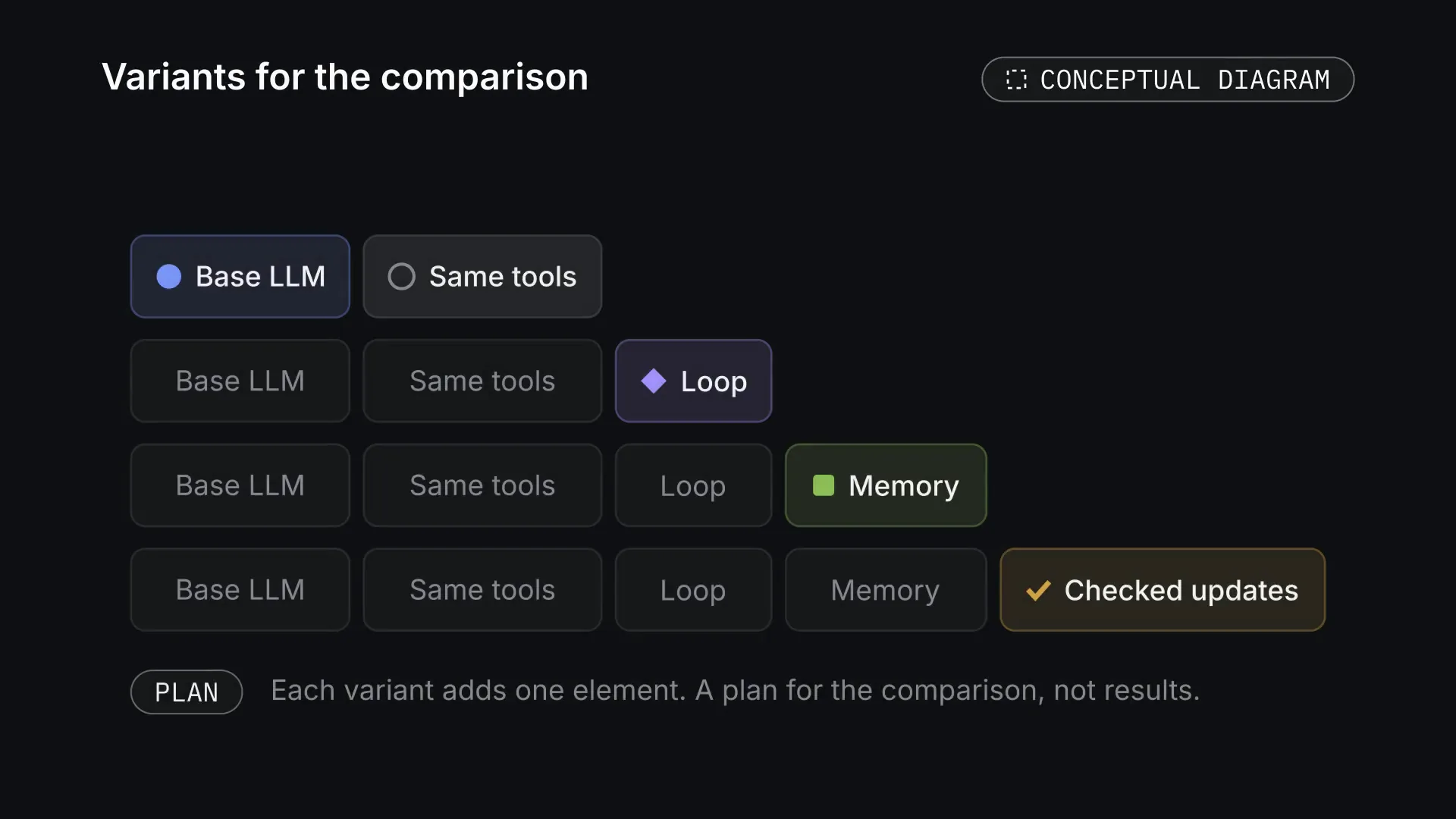
To test what each component contributes, we need variants of the system in which one essential element changes: the base LLM with the same tools; the loop without long-term memory; the loop with memory; the loop with memory and checked updates to procedures. This is a plan for the comparison, not the results of a finished experiment.
FigureVariants for the comparison. Planned variants, each adding one element: the base LLM with the same tools, the loop without long-term memory, the loop with memory, and the loop with memory and checked updates to procedures. A plan, not results. Conceptual diagram. Tap the picture to see it whole. The picture: A ladder of four rows of chips, each one chip longer. Row one: Base LLM (blue) and Same tools. Row two adds Loop (violet). Row three adds Memory (green). Row four adds Checked updates (ochre). In each row the new element is tinted with its marker; the earlier ones are plain. Below, a 'Plan' pill: each variant adds one element; a plan for the comparison, not results.
The main metric is the share of tasks that fully pass a check set in advance:
pv=N1i=1∑NYi(v),Yi(v)∈{0,1}.
v stands for the variant of the system, N for the number of tasks and Yᵢ for the result of the check. Partial completion can be scored as well, but it must not quietly turn into full success.
The difference is better computed on the same tasks:
Δ=N1i=1∑N(Yi(new)−Yi(base)).
This paired comparison shows on which tasks the new variant helped or got in the way. The estimate needs its uncertainty beside it, for example a confidence interval from a paired bootstrap over tasks. Repeated attempts at one task should not be counted as new independent tasks.
Walk-throughA paired comparison of variants · 30 sFigureA paired comparison of variants. Teaching data for four tasks: the base variant solved 2 of 4, the new one 3 of 4. The paired difference is +25 percentage points, although one task got worse. Four made-up tasks are not enough to conclude there is an improvement. Worked example · 30 s. The picture: Two formulas at the top. On the left, a small card of tuning tasks marked 'used to tune, not scored'; on the right, a table of four held-out tasks, T1 to T4. Row 'base': tick, cross, tick, cross, giving p̂ = 0.5. Row 'new': tick, tick, cross, tick, giving p̂ = 0.75. A third row shows the per-task differences 0, +1, −1, +1 and Δ̂ = +0.25 = +25 pp.
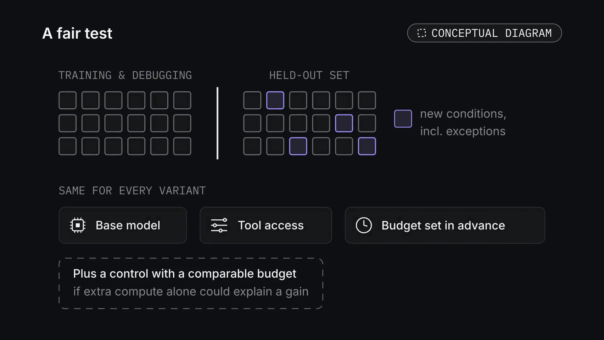
Tasks used for training and debugging have to be kept apart from the held-out set. Testing transfer will need new conditions, including exceptions to rules that were useful before. The systems being compared must have the same base model, the same access to tools and budgets set in advance. If extra compute alone could explain a gain, a separate control with a comparable budget is needed.
FigureA fair test. Training and debugging tasks stay apart from the held-out set, which includes new conditions and exceptions. Every variant gets the same base model, tool access and a budget set in advance; a compute-matched control is added if extra compute alone could explain a gain. Conceptual diagram. Tap the picture to see it whole. The picture: Top: two grids of small task squares separated by a vertical wall, 'training & debugging' and 'held-out set'; four held-out squares are violet, with a legend 'new conditions, incl. exceptions'. Below, 'same for every variant': cards Base model (chip icon), Tool access (sliders), Budget set in advance (clock). Under them a dashed card: plus a control with a comparable budget, if extra compute alone could explain a gain.
Cost is part of the result too:
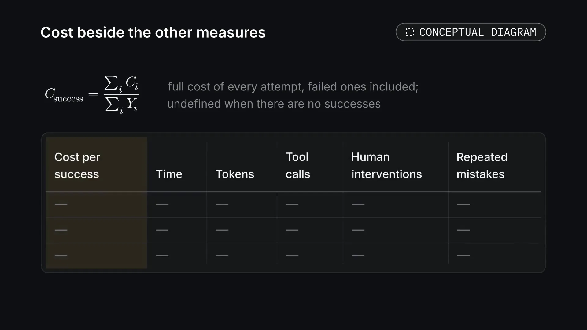
Csuccess=∑i=1NYi∑i=1NCi,i∑Yi>0.
Cᵢ is the full cost of an attempt, including a failed one. If there are no successes, the cost per success is undefined. It should be shown together with time, tokens, the number of tool calls, human interventions and repeated mistakes.
FigureCost beside the other measures. Cost per success counts the full cost of every attempt, failed ones included, and is undefined without successes. It is reported beside time, tokens, tool calls, human interventions and repeated mistakes. Conceptual diagram. Tap the picture to see it whole. The picture: The formula C_success = sum of C_i over sum of Y_i, with the note: full cost of every attempt, failed ones included; undefined when there are no successes. Below, a table header with six columns: Cost per success (tinted), Time, Tokens, Tool calls, Human interventions, Repeated mistakes; three empty rows with dashes, no values.Walk-throughThe cost of a success · 20 sFigureThe cost of a success. A teaching cost: four attempts at one unit each give 2 units per success with two successes, and about 1.333 with three. The cost of failures counts; with no successes the ratio is undefined. Worked example · 20 s. The picture: The formula at the top, with the note '1 unit per attempt'. On a panel, two rows of four flat coin tokens, one per attempt, each marked with a tick or a cross: base tick, cross, tick, cross; new tick, tick, cross, tick. Beside them: 4 / 2 = 2 and 4 / 3 ≈ 1.333. A final red-tinted line with a cross: if no attempt succeeds, the denominator is 0 and the cost per success is undefined.
When an improvement can be accepted
Being able to propose a new instruction does not mean the instruction is useful. So in the conceptual scheme an update to the system goes through an evaluation:
S′ is the proposed version of the system, for example with a changed procedure. EvalPass combines requirements chosen in advance for quality, acceptable regressions and costs. Passing this check is empirical ground for accepting the change under the given conditions, not proof that it is useful for ever.
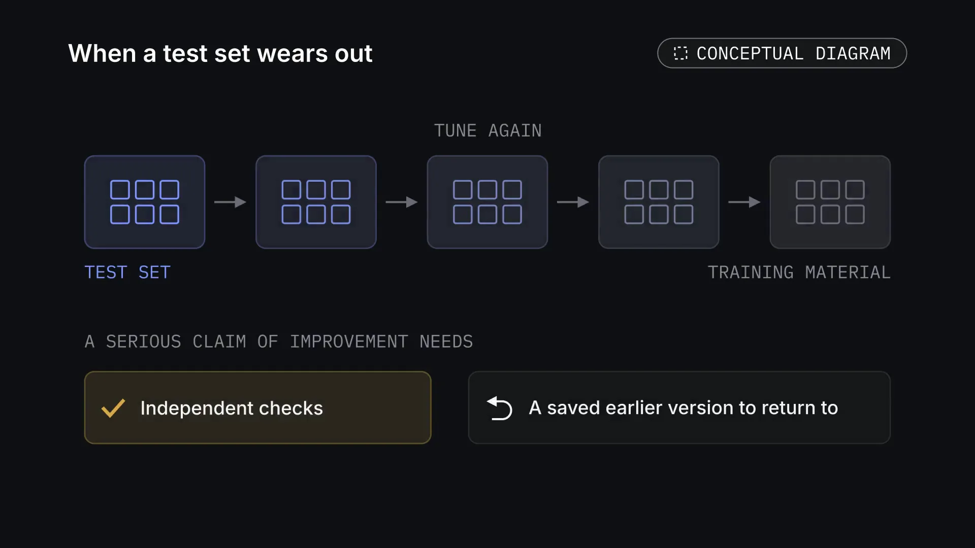
Tuning again and again on one set gradually turns it into training material. So a serious claim of improvement needs independent checks and a saved earlier version to return to.
FigureWhen a test set wears out. Tuning again and again on one set gradually turns it into training material. A serious claim of improvement needs independent checks and a saved earlier version to return to. Conceptual diagram. Tap the picture to see it whole. The picture: A row of five cards with the same grid of tasks joined by arrows, labelled 'tune again'; the cards fade from blue, 'test set', to grey, 'training material'. Below, 'a serious claim of improvement needs': an ochre card with a tick, Independent checks, and a card with an undo sign, A saved earlier version to return to.FigureChecking a proposed improvement. A conceptual check of updates: the first procedure passes the checks and becomes version 4; the next fails the regression check, so version 4 is kept. This is a rule for accepting a candidate, not a guarantee of ever-rising quality. Conceptual diagram · 26 s. The picture: The cases formula at the top. A thin version track at the bottom starts at v3, marked current. A blue-tinted candidate card 'new retry procedure' is joined by thin arrows to three check cards — quality, no regressions, cost — and gets three ochre ticks; it becomes v4 on the track. A second candidate 'shorter prompts' passes quality but gets a red cross at 'no regressions'; its trial is marked rejected and a green arrow returns to v4.
Why long work stays hard
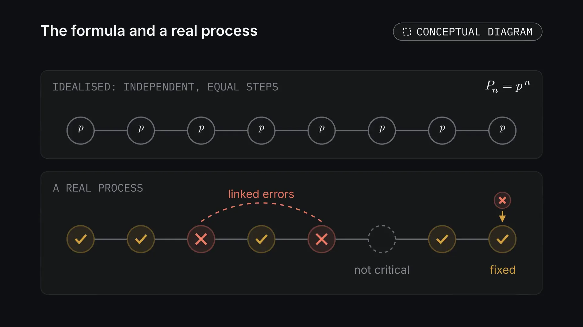
In a long chain, a small chance of error at each step can noticeably lower the overall reliability. If success requires every critical step to succeed, the chain rule of probability applies:
Pr(E1∩⋯∩En)if all conditional probabilities equal p:Pn0.99100=i=1∏nPr(Ei∣E1,…,Ei−1),=pn,≈0.366,0.999100≈0.905.
The last numbers are a teaching calculation with equal conditional probabilities, not a measurement of any model. In a real process errors are linked to each other, some can be fixed and some steps are not critical. The formula shows why checking intermediate results and recovering from failures matter for long work.
FigureThe formula and a real process. The teaching formula assumes independent steps with equal probability p. In a real process errors are linked, some can be fixed and some steps are not critical. Conceptual diagram. Tap the picture to see it whole. The picture: Top panel, 'idealised: independent, equal steps': eight identical rings each marked p joined in a line, with P_n = p^n. Bottom panel, 'a real process': a line of steps with ochre ticks; two clay crosses joined by a dashed arc, 'linked errors'; a dashed ring, 'not critical'; and a last step where a small cross above points down into a tick, 'fixed'.
The end of the animation looks at one more teaching mechanism: detecting and correcting errors. Let c be the share of wrong steps that were both detected and fully corrected. If the check does not spoil results that were right to begin with, the effective probability that a step succeeds is:
peff=p+(1−p)c=1−(1−p)(1−c).
With p = 0.99 and c = 0.9 this gives p_eff = 0.999. This is a conditional calculation, not a measurement of Sapphire: successful detection together with full correction is folded into the one value c. New errors the check itself might introduce are not counted in this simple model.
FigureThe reliability of a long chain. A teaching model: with the same conditional chance of success of 0.99 per step, a hundred steps give about 36.6%, with 0.999 about 90.5%. The last part shows the conditional effect of correcting 90% of errors with a reliable check; it is not an actual property of the system. Worked example · 28 s. The picture: Two formulas at the top. A flat line chart with thin axes and gridlines: number of steps n from 0 to 100, chance the whole chain succeeds from 0 to 100 %. A grey curve for p = 0.99 falls to 36.6 % at n = 100; a blue curve for p = 0.999 stays high and ends at 90.5 %. Then, on a card at the right, the formula p_eff = 1 − (1 − p)(1 − c) with c = 0.9, and an ochre arrow from the grey end point to the blue one: checking and recovery lift the chain.
That is why we treat Sapphire as research into how AI work is organised. It will have to be judged by how it finds errors, uses experience and copes with new tasks within given limits.
What the next entry should bring
Our long-term goal is to study the path to more general and more independent artificial intelligence. We allow that joining generation, decisions and checked experience may turn out to be part of that path. Whether such a system would be enough for AGI does not follow from our concept today.
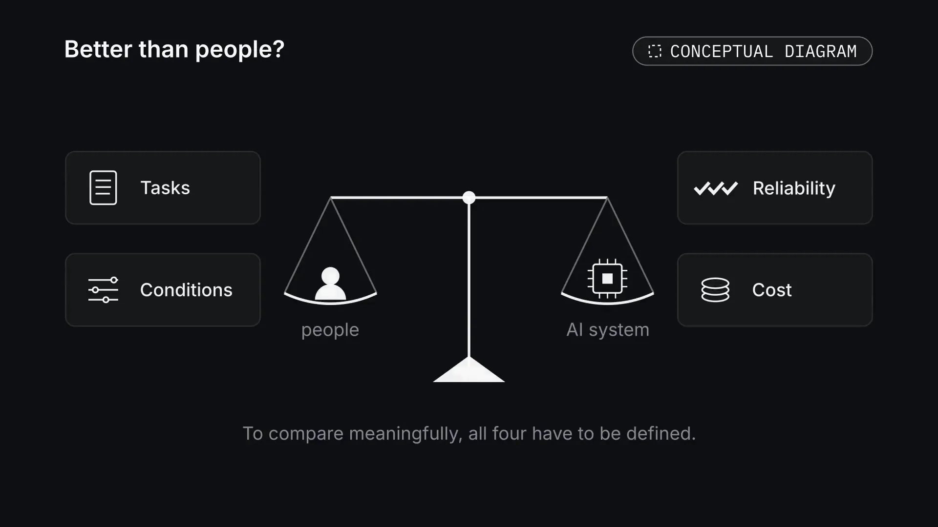
Outperforming people at particular tasks is also not the same as outperforming them across the whole range of intellectual work. To discuss that meaningfully, the tasks, conditions, reliability and cost of the comparison have to be defined. A timeline of a few months or years remains a guess, not a result of this work.
FigureBetter than people? Outperforming people means little until the comparison is defined: which tasks, under what conditions, how reliably and at what cost. Conceptual diagram. Tap the picture to see it whole. The picture: A level balance with a person pictogram on the left pan, 'people', and a chip pictogram on the right pan, 'AI system'. Two cards on each side: Tasks (page), Conditions (sliders), Reliability (three ticks), Cost (coins). Below: to compare meaningfully, all four have to be defined.
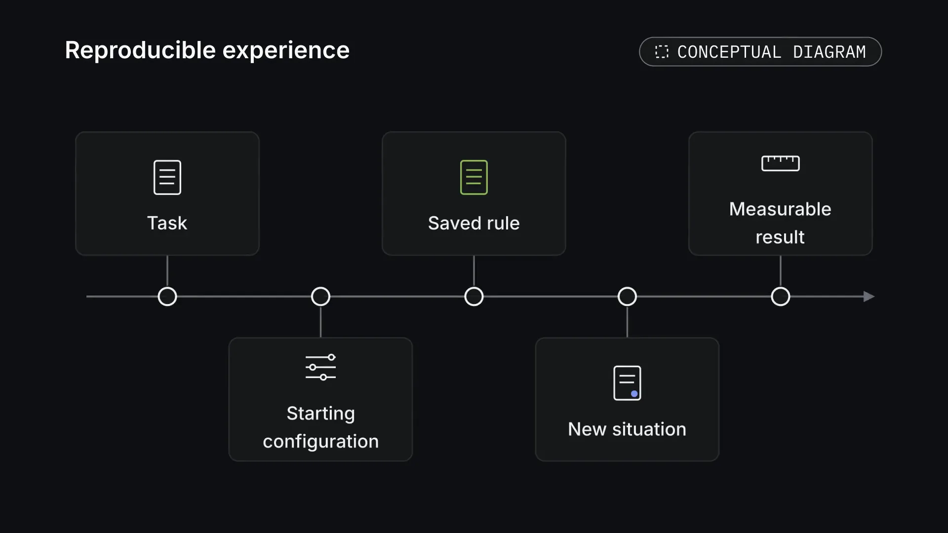
Sapphire's next real milestone is reproducible experience: a task, a starting configuration, a saved rule, a new situation and a measurable result. Most interesting is the case in which the system first made a mistake, then used checked experience and could explain the limits of where it applies. Material like that will give this research diary what we are starting it for: observations that can be discussed and checked.
FigureReproducible experience. The next real milestone is reproducible experience: a task, a starting configuration, a saved rule, a new situation and a measurable result. Conceptual diagram. Tap the picture to see it whole. The picture: A horizontal timeline with five stations; cards alternate above and below it: Task (page), Starting configuration (sliders), Saved rule (green page), New situation (page with a blue dot), Measurable result (ruler).
Sources
Morris et al. Levels of AGI for Operationalizing Progress on the Path to AGI. 2023, with later revisions. https://arxiv.org/abs/2311.02462
METR. Task-Completion Time Horizons of Frontier AI Models. The page is marked as no longer actively updated; the last stated update is 8 September 2026. https://metr.org/time-horizons/
Archival pictures in the collages: [Card catalog], Harris & Ewing, 1932, Library of Congress (no known restrictions); [Card sorter for tabulating machine at the US Census Bureau], Harris & Ewing, 1940, Library of Congress (no known restrictions); CENSUS BUREAU. DEPARTMENT OF COMMERCE. TABULATING MACHINE, Harris & Ewing, 1917, Library of Congress (no known restrictions); Corundum (GeoDIL number - 1438), Nessa Eull, 2001, Wikimedia Commons (CC0).